Vegetable Degree-day Models: An Introduction for Farmers and Gardeners

For centuries, farmers have recognized the relationship between temperature and plant development. The growth rate of many plants, insects and fungi is strongly temperature-dependent. This allows us to predict the development rates of many organisms using development models based on the accumulation of heat units, known as degree-days, during a growing season.

As early as the 18th century, scientists such as René A. F. de Réamur were measuring the relationship between mean daily temperatures and crop development. In the mid-20th century, agricultural researchers introduced the concepts of upper and lower developmental thresholds and various methods of calculating degree-days, or DDs. DDs measure the amount of heat accumulated over time. These concepts provided a scientific framework for developing modern DD models. These phenology models predict the timing of events in an organism’s development.

Many factors other than time and temperature can influence the development rate of plants, including water, nutrients and pests. DD models only account for time and temperature, but they are usually more accurate than calendar days, which are based on time alone.

Farmers and gardeners can use this set of crop and pest development models to predict harvest dates and other important events in select crops and annual weeds. This guide also introduces growers to the OSU Croptime DD modeling project.

What are temperature thresholds?

Mammals regulate their body temperatures internally using energy from food. The body temperatures of plants, insects and fungi are more similar to ambient air temperature. That’s why our normal body temperature is about 98.6°F regardless of the weather, and the body temperature of an insect is about 50°F when the temperature in its environment is about 50°F. Generally, the development rate of an organism is faster at warm temperatures and slower at cooler temperatures. There are lower and upper limits to this relationship, however, so DD models use temperature thresholds to account for these limits.

Lower thresholds are the temperatures at which development rates approach zero or stop entirely. This value for plants, depending on the type, usually ranges from 32°F to 55°F. Upper thresholds, while not always needed in DD models, are similar in setting an upper temperature limit for development. Usually, rather than signifying that development stops at the upper threshold, this value is used to denote that the development rate stops increasing above the upper threshold. When temperatures are close to the lower threshold, DDs accumulate slowly, and DD accumulation is fastest at warmer temperatures near the upper threshold. Temperature thresholds are identified in controlled temperature experiments, or with data from field trials. They usually don’t vary much within a crop species or group of closely related species or varieties.

See Appendix for the lower and upper thresholds used in Croptime models.

What are degree-days?

Degree-days provide a way to estimate the development rate of plants, insects, fungi and other organisms using hourly or daily maximum and minimum temperatures. DDs measure the amount of heat accumulated over time. They can be calculated in many different ways. The simplest way to calculate DD accumulation is the simple average method:

(Tmin + Tmax)/2 – Tbase = degree-days

Tmin = minimum daily temperature

Tmax = maximum daily temperature

Tbase = lower development threshold

For example, assume that a crop’s lower threshold is 50°F and its upper threshold has not been determined or is very high and therefore not used. On a day with a high of 90°F and a low of 40°F, DDs are calculated as:

(40 + 90)/2 – 50 = 15 degree-days

For some crops such as sweet corn, the night-time low temperature is not very important because the plant shuts down at night. For these crops, an alternative temperature substitution DD calculation method usually performs more accurately than the simple average methods. This method is known as the “Corn Growing DD Method” or the “threshold substitution method.” If the daily high or low temperatures are above or below the thresholds, they are substituted using the threshold. For example, using the same daily temperature values as above, a lower threshold of 50°, and adding an upper threshold (used for corn) of 86°, we would reset the Tmin from 40 to 50 and the Tmax from 90 to 86 and calculate:

(50 + 86)/2 – 50 = 18 degree-days

Degree-day calculation methods

The simple average method nicely illustrates the DD concept. More sophisticated triangle and sine methods are usually more accurate. The sine method, for example, calculates the area under the curve between the minimum and maximum thresholds as shown by the shaded area in Figure 1. Croptime models and most insect DD models used in Oregon use a version of this known as the “single sine DD method.” Most models use daily minimum and maximum temperatures, but some have been developed using temperatures calculated hourly, for degree-hours. When divided by 24, degree-hours are another DD calculation method. Some instruments known as bioaccumulators and weather stations with custom software can accumulate DDs with precision to the minute or less. The different methods of calculating DDs are typically not interchangeable. Users of DD models must use the calculation method that was used to develop the model, or recalibrate the model. For example, if a model specifies a “single sine method,” then subsequent model runs should also use that calculation method. The Croptime website automatically selects the correct calculation method for Croptime models. See the Appendix or online model documentation to confirm the calculation method used for each crop if you use these models outside the Croptime platform.

Using degree-day models to schedule planting and harvest

DD models can predict harvest dates more accurately than rough guidelines such as calendar days provided in seed catalogs. Increased prediction accuracy may help ensure a consistent supply of crops when planning crop successions.

During the growing season, model predictions usually become more accurate as harvest approaches, and short- and long-term forecasts are replaced with weather data from the local weather station. Midseason model runs may help when communicating with buyers and planning farm work crews and crop sales. If you plant earlier in the year, it’s usually cooler, so you accumulate DDs more slowly than if you plant later in the season. The same is true for warmer vs. cooler years.

Figure 2 shows the difference in predicted days to maturity for ‘Arcadia’ broccoli grown in Aurora, Oregon (66 to 103 days). There were 20 to 32 days difference in the time to maturity within a season, depending on the planting date, and 0 to 14 days difference in the time to maturity at the same planting date in different seasons. On average, ‘Arcadia’ broccoli took seven days longer to reach maturity after the same planting date in cooler years (2011–2012) than in warmer years (2013–2015).

Using degree-day models to help manage weeds

Farmers and agricultural scientists have long recognized that when weeds are allowed to produce viable seed, the weed seed bank is increased, leading to an increase in weed management costs that can last for many years.

“Weed seed rain” is a phrase used to describe seed dispersal from weeds that are allowed to go to seed in a field. If growers can predict when problem weeds in their fields will set viable seed, they can avoid weed seed rain by killing weeds earlier.

Early season weed control is important and cost-effective, especially when you can control weeds mechanically or with herbicides. Some weeds inevitably escape early season control. As crops mature, mechanical weeding and herbicide applications become impractical.

Hand weeding is an expensive management option, but if escapees are likely to set viable seed, it is often worth the investment in order to reduce weed seed rain.

Croptime weed models for hairy nightshade, redroot pigweed and lambsquarter predict the time from cotyledon emergence to first viable seed set. If these weeds are important in your fields, you can use the models to avoid weed seed rain.

To use Croptime weed models, monitor your fields to identify when cotyledons emerge, and use that as the start date for the model. If you didn’t collect this information, estimate emergence after your last cultivation. For example, estimate that weeds will emerge three to seven days later.

What is Croptime?

The development of the internet and the expansion of automated weather station networks in the last few decades have allowed scientists to develop decision support tools for growers and other agricultural professionals. These tools predict the development, or phenology, of insects, diseases, weeds and crops. Over time, these tools are becoming more extensive and user-friendly.

The OSU Croptime project is developing DD models useful for vegetable growers. The OSU Oregon IPM Center’s phenology website links to more than 32,000 automated weather stations throughout the U.S., and hosts more than 150 pest and crop models. The Croptime model platform is for vegetable farmers and gardeners. Croptime currently hosts 29 vegetable DD models and three summer annual weed models (see Appendix).

How can I use Croptime models?

Please see the “Quick Guide” brochure and how-to video on the Croptime website.

Click on the “Croptime Calculator” button to run models from your computer or tablet. This version allows you to enter up to four start dates at a time. An optional registration survey will appear when you go to the Calculator.

You can also run the Croptime models from a mobile device.

Steps to run a model

1. Choose a local weather station, either by entering a ZIP code or name of a town or city, or by navigating in the map and clicking on a pin representing an automatic weather station. Choose a station near your field that has a similar elevation. If you get a bad data alert in bold red font, choose another nearby station.
2. Select the specific crop and variety of interest.
3. Enter up to four planting dates (only one allowed for the mobile app version).
4. Choose your long-term forecast type and model output format.
5. Click on the “run model” button (desktop computer version) or the “Output” and “Graph” tabs (mobile app version) to see model predictions.

Croptime DD models predict growth stages (such as harvest or seed-set) using weather data from the weather station you select. The website uses recorded weather data up to the day before the model run. Short-term forecasts from the National Weather Service predict temperatures at the weather station for seven days into the future.

Within the “Forecast type” dropdown menu, you can select from a range of options to predict temperatures at that weather station more than seven days into the future. Options include 10-year averages, 30-year averages, last year’s data, data from two years ago and climate model predictions for that weather station. The “NMME” extended seasonal forecast takes into account factors such as ocean temperatures that are more accurate than historical averages.

Output options for the models include “condensed” (default), which only displays data from days when an event like harvest is predicted. If you select “no,” the uncondensed version displays data for every day of the model run. “Daylength” calculates the daylength each day at the chosen weather station; the default is to display daylength. You can select a “Critical Daylength” if that is important and known for the crop model. Choose the critical hours from the dropdown menu.

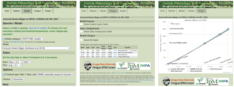
Figure 3 shows an example of the model Input, Output and Graph screens using ‘Green Magic’ broccoli transplanted on Feb. 1.

How accurate are Croptime models?

Croptime aims to provide DD models that are easy to use, so that you can predict harvest dates more accurately than with calendar-day predictions.

Generic calendar-day predictions that are sometimes shown in catalogs are not very reliable for predicting harvest dates, unless you live near where those predictions were developed. They do indicate which varieties take longer to mature in that catalog.

Custom calendar-day predictions from your farm records can be fairly accurate. Depending on the crop and the planting date, they are sometimes as accurate as DD models.

Croptime models predict DDs to maturity using data from weather stations near your farm, and National Weather Service forecasts for that weather station. Long-term temperature forecasts are based on historical averages or climate models, depending on the option you choose. They are most useful when scheduling your planting dates. Our hypothesis is that DD models are more accurate than generic calendar day predictions.

The tables in the Appendix show average days to maturity and DDs to maturity, and their relative accuracy in days using the data we collected to develop these models. For example, sweet corn (all varieties in our studies, Appendix), had an accuracy range from plus or minus 1.5 days to 22 days using calendar days observed during our research. Using the degree-day models, sweet corn accuracy ranged from plus or minus 0.3 days to 3.1 days.

Croptime models might not be as accurate as more sophisticated models that include factors such as light intensity, moisture, humidity, soil temperature, competition or pest damage.

The overall objective in the Croptime project is to develop numerous relatively simple, yet easy-to-use DD models for popular varieties that can help growers optimize their vegetable production operations.

Horticultural practices and Croptime models

Horticultural practices may influence the number of days to maturity predicted by DD models. Three examples include transplanted crops, plastic mulch and high tunnels.

• Transplanted and direct-seeded crops: We are developing different Croptime models for transplanted and direct-seeded crops.
• Plastic mulch and bare ground production: Croptime models assume bare ground production. We have not observed statistically significant differences in the development rates of tomato and pepper varieties grown with black plastic mulch compared to bare ground, but we have seen yield increases with black plastic mulch.
• High tunnels, low tunnels and row covers: These protections change ambient temperature. In order to use Croptime models in these conditions, you would have to collect your own temperature data rather than using data from your local weather station.

Can I use Croptime models in other regions?

Croptime was created with the primary aim of providing predictions of crop developmental stages for the maritime Pacific Northwest. Our DD models are being developed with data from field trials in irrigated vegetable production systems mainly in the Willamette Valley of Oregon. We welcome collaborators from other regions.

In the Willamette Valley, we have a cool Mediterranean climate with relatively cool, dry summers and generally mild, wet winters. From May 1 to Oct. 31, daily minimum temperatures are usually 40°F to 55°F, daily maximum temperatures are usually 60°F to 90°F, and average daily temperatures are usually 50°F to 70°F. Day length varies from 10 to 17 hours. We normally have about 10 inches of rain from May 1 to Oct. 31.

If you are using Croptime models in climates that are different from the Willamette Valley, local weather patterns and other factors might influence plant development rates in your area and reduce the accuracy of these DD models. For example, in hotter climates, upper thresholds may be more important and affect model accuracy. Longer or shorter days, different light intensities or precipitation, and other variables might also influence crop development rates.

Assuming that the lower and upper threshold temperatures used in the Croptime models are accurate, degree-days to maturity can still vary in different climates. You can assess the accuracy of Croptime models in different regions by:

1. Recording your planting or seeding date.
2. Making note of the dates that plants reach the key growth stages predicted in the model. Use the growth stage descriptions provided in the Appendix and in the Growth Stage Guide on the Croptime website..
3. Comparing Croptime predictions at the end of the season with your observations. Early season Croptime predictions also include inaccuracies inherent with weather forecasts and climate models.

If you collect these records a few times, you can adjust the degree days to maturity based on the averages obtained in your area and use the degree-day calculator to predict time to maturity.

Croptime modeling methods

We are determining thresholds and time to maturity based on lowest error methods, mainly using the statistical method known as the coefficient of variation (C.V.). A single data set for these calculations consists of one variety grown in one location at one planting date. We use seven to 15 data sets (specific variety, location and planting date) to determine upper and lower thresholds for crops grown in western Oregon, and three to five data sets to determine time to maturity for additional cultivars of the same crop. We select thresholds that are supported by our data and are consistent with scientific literature.

Our standard approach is to use a single sine curve with horizontal cutoff as our DD calculation method, which has been the standard recommendation for pest models by the University of California at Davis. See “Degree-day calculation methods” and the University of California Statewide IPM Program, for more information about calculation methods and cutoff methods. We also test other calculation methods when we are developing Croptime models.

Resources and next steps

The Croptime home page includes how-to instructions, a video tutorial and educational slides. We have also posted a growth stage guide for the crops that we are currently modeling. We plan to publish new DD models for spinach, lettuce, carrots, parsnip, cauliflower, cabbage, kale and summer squash in the future. We are also interested in collaborating with farmers, seed companies and researchers to develop new Croptime models. Please contact the authors if you would like more information about this ongoing project or are interested in collaborating.

Appendix: Croptime vegetable phenology models

Croptime includes DD models for transplanted broccoli, transplanted and direct-seeded cucumber, direct-seeded snap beans, transplanted and direct-seeded sweet corn, and transplanted sweet pepper and tomato varieties. Weed models include hairy nightshade, lambsquarter and redroot pigweed. Model paremeters and key growth stages are described below.

Broccoli degree-days (transplanted)

Degree-day model summary for broccoli varieties (Brassica oleracea) transplanted at 2–4 true leaves using a 32°F lower threshold, a 70°F upper threshold, and single sine calculation method with a horizontal cutoff.

Table 1. Model parameters for four transplanted broccoli cultivars

Variety	50% head initiation (DDs)	First harvest (DDs)	Early flowering (DDs)	DD model accuracy1 (days)	Observed days to early flowering2	Calendar-day accuracy1 (days)	Number of data sets3
Arcadia	1674	2281	2672	±2.5	86	±7.5	8
Emerald Pride	1565	2151	2518	±6.4	77	±11	5
Green Magic	1458	2103	2456	±4.1	81	±23	10
Imperial	1753	2383	2688	±4.6	85	±6.5	4

1 Accuracy calculated as mean absolute difference is estimated from original DD or calendar-day data, not from independent verification data.

2 Observed average days from transplant to early flowering in our data sets. Early flowering is used here because it was a more distinct growth stage than harvest for broccoli.

3 One data set consists of plant development observations at one location and one planting date. Most data was collected in the Willamette Valley from 2013 to 2015.

Cucumber degree-days

Degree-day model summary for cucumber varieties (Cucumis sativus) direct seeded and transplanted at two true leaves using a 50°F lower threshold and 90°F upper threshold, and single sine calculation method with a horizontal cutoff.

Table 2. Model parameters for one transplanted and six direct-seeded cucumber cultivars

Variety	Type	Direct -seeded or transplanted	2 true leaves (DDs)	Early flowering (DDs)	First harvest (DDs)	DD model accuracy1 (days)	Observed days to harvest2	Calendar- day accuracy1 (days)	Number of data sets3
Cobra	Slicing	DS	339	665	964	±2.5	57	±7	11
Dasher II	Slicing	DS	365	731	1060	±1.8	55	±3.5	5
Marketmore 76	Slicing	DS	364	784	1211	±1.1	67	±10	8
Marketmore 76	Slicing	TP	na	344	805	±1.9	46	±7	7
Extreme	Pickling	DS	366	692	946	±1.2	50	±6	5
Supremo	Pickling	DS	366	677	981	±0.8	52	±5	5
Zapata	Pickling	DS	380	688	984	±2.7	56	±7.5	6

1 Accuracy calculated as mean absolute difference is estimated from original DD or calendar-day data, not from independent verification data.

2 Observed average days from direct seed or transplant to harvest in our data sets.

3 One data set consists of plant development observations at one location and one planting date. Most of our data was collected in the Willamette Valley from 2013 to 2015.

Snap bean degree-days

Degree-day model summary for direct-seeded varieties of snap beans (Phaseolus vulgaris) using a 40° F lower threshold, a 90°F upper threshold and single sine calculation method with a horizontal cutoff.

Table 3. Model parameters for three direct-seeded snap bean cultivars

Variety	First trifoliate leaf (DDs)	First open flower (DDs)	Harvest (DDs)	DD model accuracy1 (days)	Observed days to harvest2	Calendar-days accuracy1 (days)	Number of data sets3
5360	601	1148	1630	±5.1	58	±10	9
Provider	608	1094	1681	±1.5	61	±2	4
Sahara	526	1248	1805	±2.0	64	±3	4

1 Accuracy calculated as mean absolute difference is estimated from original DD or calendar-day data, not from independent verification data.

2 Observed average days from direct seed to harvest in our data sets.

3 One data set consists of plant development observations at one location and one planting date. Most of our data was collected in the Willamette Valley from 2013 to 2015.

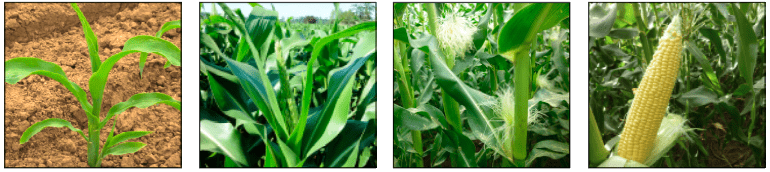
Sweet corn degree-days

Degree-day model summary for varieties of sweet corn (Zea mays) direct seeded and transplanted at one to two true leaves. For fresh market varieties, we used a lower threshold 44°F; for processing varieties we used a lower threshold 50°F. We used an upper threshold of 86°F using the corn GDD calculation method for all varieties.

Table 4. Model parameters for three transplanted and five direct-seeded sweet corn cultivars

Variety	Direct-seeded or transplanted	5 true leaves (DDs)	5-inch tassel (DDs)	95% silk (DDs)	Fresh harvest (DDs)	Process harvest (DDs)	DD model accuracy1 (days)	Observed days to harvest2	Calendar-days accuracy1 (days)	Number of data sets3
Jubilee	DS	308	883	1145	1539	1597	n/a	n/a	n/a	n/a
Luscious	DS	442	1084	1414	1854	N/A	±1.9	78	±6	7
Luscious	TP	451	1123	1516	1934	N/A	±0.3	81	±4	3
Sugar Pearl + Temptation	DS	446	982	1342	1883	N/A	±1.5	75	±1.5	4
Sugar Pearl + Temptation	TP	409	1099	1555	2014	N/A	±2.6	81	±4	5
4001	DS	390	794	1075	1444	1644	±1.8	105	±22	4
Kokanee	DS	300	845	1130	1498	1650	±3.1	96	±8	8

1 Accuracy calculated as mean absolute difference is estimated from original DD or calendar-day data, not from independent verification data.

2 Observed average days from direct seed or transplant to fresh market harvest in our data sets.

3 One data set consists of plant development observations at one location and one planting date. Most of our data was collected in the Willamette Valley from 2013-2015.

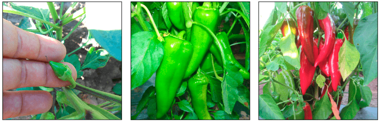
Sweet pepper degree-days

Degree-day model summary for varieties of sweet pepper (Capsicum annuum) transplanted at four to seven true leaves using a 52°F lower threshold, a 100°F upper threshold and single sine calculation method with a horizontal cutoff.

Table 5. Model parameters for four transplanted sweet pepper cultivars.

Variety	Fruit set (DDs)	First green harvest (DDs)	First ripe harvest (DDs)	DD model accuracy1 (days)	Observed days to harvest2	Calendar- day accuracy1 (days)	Number of data sets3
Bell King	739	1447	1998	±5.4	84	±8	7
Gatherer’s Gold	575	1212	1692	±3.4	79	±16.5	9
King Arthur	608	1321	1767	±11.7	73	±9	6
Stocky Red Roaster	586	1211	1682	±2.0	78	±16	10

1 Accuracy calculated as mean absolute difference is estimated from original DD or calendar-day data, not from independent verification data.

2 Observed days from transplant to first green harvest in our data sets.

3 One data set consists of plant development observations at one location and one planting date. Most of our data was collected in the Willamette Valley from 2013 to 2015.

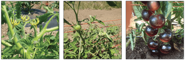
Tomato degree-days

Degree-day model summary for varieties of tomato (Solanum lycopersicum) transplanted at three to five true leaves using a 45°F lower threshold, a 92°F upper threshold and single sine calculation method with a horizontal cutoff.

Table 6. Model parameters for four transplanted tomato cultivars

Variety	First flower (DDs)	2-inch fruit growth (DDs)	Harvest (DDs)	DD model accuracy1 (days)	Observed days to harvest2	Calendar-day accuracy1 (days)	Number of data sets3
Big Beef	505	1050	1970	± 3.3	84	±3.5	8
Indigo Rose	590	1094	2010	±2.6	85	±8	6
Monica	600	1091	1976	±2.2	83	±7	6
New Girl	498	1029	1844	±4.5	80	±9.5	11

1 Accuracy calculated as mean absolute difference is estimated from original DD or calendar-day data, not from independent verification data.

2 Observed average days from transplant to first ripe harvest in our data sets.

3 One data set consists of plant development observations at one location and one planting date. Most of our data was collected in the Willamette Valley from 2013 to 2015.

Summer annual weed degree-days

Weed development for common weeds of vegetables with varying upper and lower thresholds. Degree-days calculated using single sine calculation method with a horizontal cutoff.

Table 7. Model parameters for three common annual summer weed species

Weed species	Upper threshold (degrees Fahrenheit)	Lower threshold (degrees Fahrenheit)	First seed (DDs)	Lower 95% confidence interval1 (DDs)	Upper 95% confidence interval1 (DDs)	Number of data sets3
Hairy nightshade2	95	40	1811	1668	1954	8
Lambsquarter2	95	42	1462	1360	1564	7
Redroot pigweed2	89	46	1078	1004	1152	7

1 95% probability that the confidence interval will contain the mean first viable seed for the population of weeds.

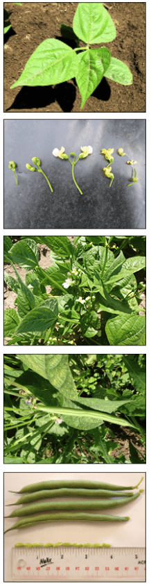
2 Top to bottom: Solanum sarrachoides, Chenopodium album and Amaranthus retroflexus.

3 One data set consists of plant development observations at one location and one planting date. Most of our data was collected in the Willamette Valley from 2013 to 2015.

© 2021 Oregon State University.

Extension work is a cooperative program of Oregon State University, the U.S. Department of Agriculture, and Oregon counties. Oregon State University Extension Service offers educational programs, activities, and materials without discrimination on the basis of race, color, national origin, religion, sex, gender identity (including gender expression), sexual orientation, disability, age, marital status, familial/parental status, income derived from a public assistance program, political beliefs, genetic information, veteran’s status, reprisal or retaliation for prior civil rights activity. (Not all prohibited bases apply to all programs.) Oregon State University Extension Service is an AA/EOE/Veterans/Disabled.