
Summary
Applying too much or too little water is one of the most common irrigation management challenges.
Excess irrigation can:
- Leach nutrients beyond the root zone
- Increase runoff and soil erosion
- Promote crop diseases
- Waste water and energy, increasing costs
Insufficient water leads to:
- Crop stress
- Reduced yields
- Diminished crop quality
Benefits of irrigation water scheduling
Proper irrigation scheduling:
- Applies water only when needed
- Reduces nutrient leaching
- Minimizes runoff and deep percolation
- Improves crop yield and quality
- Reduces pumping time and energy use
- Improves long-term soil health
Effective scheduling maximizes return per unit of water applied.
Irrigation scheduling is the process of determining when to irrigate and how much water to apply based on crop demand and soil water availability. Effective scheduling requires knowledge of:
- How much water your crop needs = Crop water use (evapotranspiration, or ET)
- How much water your soil can hold = Soil water-holding capacity
- Soil depth management = Rooting depth
- How much water and how efficiently your irrigation system applies it = Irrigation system application rate and efficiency
With basic field information and a few calculations, irrigators can significantly improve water-use efficiency, crop performance and energy management within their operations.
What do you need to get started?
Irrigation scheduling is manageable when broken into key components. To develop a schedule, you will need to know:
- The available water capacity of your soil
- The ffective rooting depth of the crop
- The maximum allowable depletion for the crop
- The application rate of your irrigation system
- Your irrigation system’s efficiency
Together, these values determine how much water can be stored, how much can be safely depleted and how much must be applied to refill the root zone.
1. The available water capacity of your soil
The first step is determining how much water your soil can store within the crop root zone.
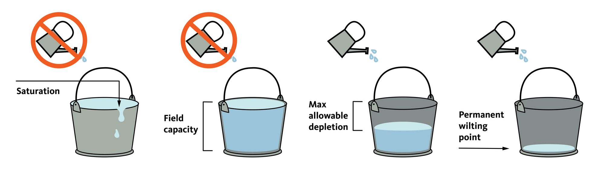
Think of the soil as water reservoir or a bucket. The water in the bucket represents the water status in the soil profile (Figure 1).
- Immediately after heavy irrigation or a rainfall event, all soil pores (large and small) may be filled with water. This condition is called saturation. Under saturated conditions, gravitational water drains rapidly through the largest pores and is generally not retained in the root zone. Thus, it is unavailable to plants. This is when the bucket overflows.
- After gravitational drainage slows significantly, the soil reaches field capacity. At this point, water is held in smaller pores by capillary forces and is generally available for plant uptake.
- As the soil continues to dry, water is held increasingly tightly to soil particles. Plants must exert greater suction to extract water as soil-water tension (matric potential) increases. Eventually, the soil reaches the permanent wilting point — the point at which water remains in the soil but is held too tightly for plants to extract sufficient water to recover from wilting.
- The difference in soil water content between field capacity and permanent wilting point is called the available water capacity.
Note: Although available water capacity represents plant-available water, not all water within this range is equally accessible. As soil dries, plants must work harder to extract water. For this reason, irrigation is typically scheduled at the maximum allowable depletion threshold to avoid plant stress and prevent the soil from approaching the permanent wilting point.
Available water capacity varies by soil texture and structure. Generalized available water capacity values for different soil textures are provided in the sidebar about soil texture and typical available water capacity.
If you know your soil texture, you may use the information in the sidebar to estimate available water capacity. For field-specific values, use the National Resources Conservation Service Web Soil Survey to identify soil map units and obtain soil physical property data, including:
- Water content at field capacity
- Water content at permanent wilting point
- Available water capacity
See the step-by-step user guide on how to use the Web Soil Survey.
Important: If your field contains multiple soil map units, avoid relying on a single “average” soil. Instead, choose one of the approaches below:
- Good — simple and conservative: Base irrigation timing on the soil map unit with the lowest available water capacity within the actively irrigated area, then manage application depth so you don’t exceed infiltration capacity (to reduce runoff/deep percolation). This reduces the risk of crop stress in the “driest” parts of the field typical of coarser or shallower soils.
- Better — zone-based management: If soil differences are consistent across the field, manage irrigation in zones (separate sets, valves, blocks or variable rate irrigation prescriptions). Schedule each zone using its own soil texture/available water capacity and effective rooting depth. This improves uniformity of crop water status and reduces overwatering in areas with higher available water capacity.
- Best — data-verified zoning: Use soil maps plus field verification (soil probes, infiltration observations, yield/Normalized Difference Vegetation Index patterns, and/or soil moisture sensors) to define management zones. Place at least one sensor in a zone with lower available water capacity and one in a higher capacity zone to confirm depletion patterns and refine timing.
2. Crop’s effective rooting depth
Once you know the available water capacity of your soil, the next step is determining how much of that water can be stored within the crop’s effective rooting depth.
Effective rooting depth is defined as the portion of the soil profile where approximately 70% of water uptake occurs (Figure 2). This depth is typically less than the maximum observed rooting depth.
Effective rooting depth varies by:
- Crop species
- Soil conditions
- Root development stage
- Compaction layers or restrictive horizons
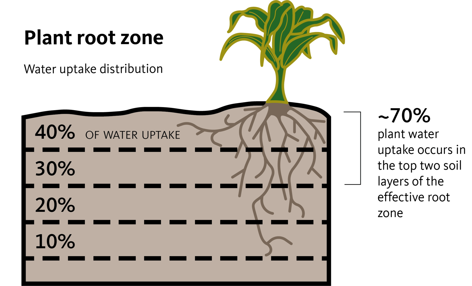
For many crops at maturity, effective rooting depth is often about one-half to two-thirds of the maximum rooting depth. However, this is a guideline rather than a strict rule.
Seasonal changes in rooting depth
For annual crops, effective rooting depth increases as roots develop during the growing season. Early in the season, the crop may extract water only from shallow depths. As roots extend deeper, a larger soil volume contributes to plant-available water.
Irrigation scheduling should account for this seasonal change in rooting depth. Scheduling based on full-season root depth early in the season may result in overestimation of available water and delayed irrigations that stress young plants.
Estimating effective rooting depth in the field
Table 1 provides typical effective rooting depths for specific crops at maturity.
For field-specific estimates:
- Carefully excavate several representative plants keeping the roots intact.
- Measure the maximum root depth.
- Multiply the average maximum root depth by approximately 0.7 (70%) to estimate rooting depth.
Because root growth varies among plants and across field conditions, assess multiple plants and use an average value. Also consider soil limitations, such as compacted layers, shallow restrictive horizons or high water tables that may limit functional rooting depth.
|
Crop (established) |
Effective rooting depth (feet) |
Maximum allowable depletion (%) |
|---|---|---|
|
Alfalfa |
4.0 | 60 |
|
Beans |
2.0 | 50 |
|
Corn |
3.0 | 50 |
|
Grapes |
3.0 | 65 |
|
Orchard |
3.0 | 50–65 |
|
Potato |
2.0 | 30–40 |
|
Pasture/hay |
2.0 | 60 |
|
Small grains |
3.0 | 50 |
3. Maximum allowable depletion
Once we know how much water can be stored within the effective rooting zone (our bucket), we need to determine the amount of water that can be depleted before irrigation is required to avoid crop water stress.
Maximum allowable depletion, or MAD, is the fraction of plant available water that can be removed from the soil through evapotranspiration (the evaporation from the soil and leaf surfaces plus the transpiration from the plant) before crop stress (Figure 3).
Maximum allowable depletion is expressed as a percentage of available water storage and depends on:
- Crop species
- Growth stage
- Rooting depth
- Economic value of the crop
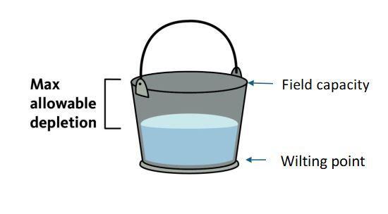
Table 1 shows recommended maximum allowable depletion values for certain crops. Generally, maximum allowable depletion values are 30%–40% for high-value, shallow-rooted crops; 50%–55% for deep-rooted crops; and 60%–65% for low-value crops such as pastures.
4. Application rate of your irrigation system
To determine the application rate of your irrigation system, you must know how much water your irrigation system applies over a specific timeframe. Application rate allows you to adjust irrigation duration and/or frequency so that you are replenishing the water depleted from the soil through evapotranspiration.
Two key pieces of information are required:
- Flow rate: volume of water delivered through a system or emitter over a specific time.
- Set time: the duration of the irrigation event.
Flow rate
Flow rate is typically expressed in gallons per minute (gpm).
For most sprinkler systems:
- Wheel line, hand line or solid set systems: Determine the average flow rate (gpm) per sprinkler.
- Pivot and linear systems: The total system flow rate is the sum of the rates of all the nozzles’ on the entire pivot or linear system.
Table 2 provides flow rates for various nozzle sizes at different operating pressures.
To determine your nozzle flow rate:
- Identify nozzle size (diameter) on your sprinkler.
- Measure the operating pressure at the sprinkler.
|
Nozzle size (inch) |
|
||||
|---|---|---|---|---|---|
| 30 | 40 | 50 | 60 | 70 | |
|
3/32 |
1.4 | 1.7 | 1.9 | 2.0 | 2.1 |
|
1.8 |
2.6 | 3.0 | 3.3 | 3.5 | 3.8 |
|
9/64 |
3.3 | 3.7 | 4.2 | 4.5 | 4.9 |
|
5/32 |
3.9 | 4.5 | 5.0 | 5.4 | 5.8 |
|
11/64 |
4.7 | 5.4 | 6.0 | 6.6 | 7.1 |
|
3/16 |
5.5 | 6.3 | 7.0 | 7.7 | 8.3 |
|
13/64 |
6.4 | 7.4 | 8.2 | 9.0 | 9.7 |
|
7/32 |
7.4 | 8.6 | 9.6 | 10.5 | 11.3 |
Source: Morris, 2023
Pressure may be measured using:
- A calibrated pressure gauge installed on the lateral near the sprinkler, or
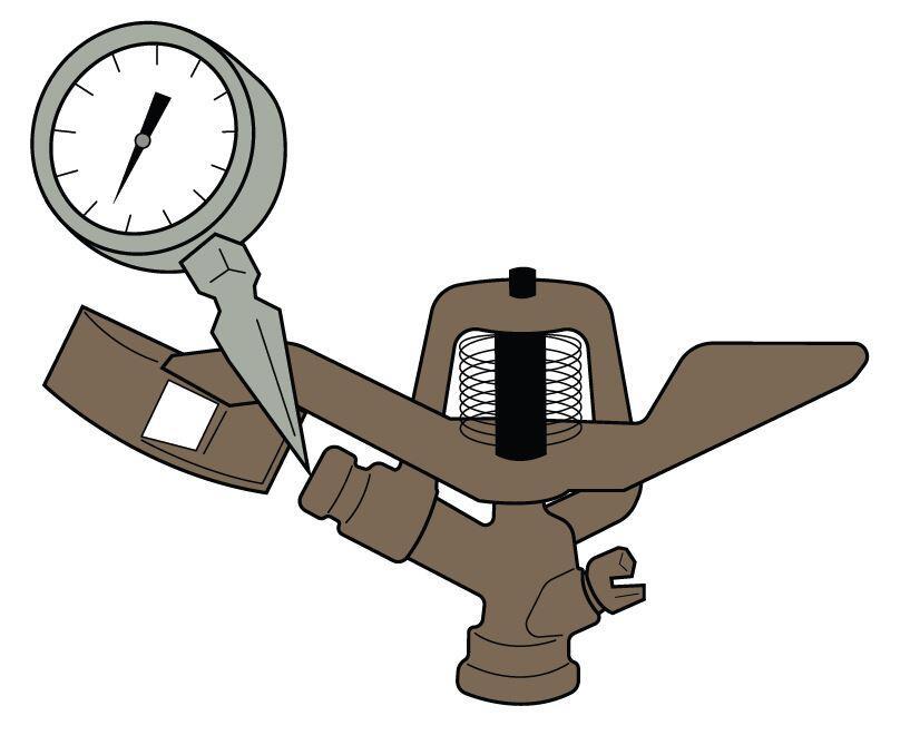
- A pitot tube inserted into the sprinkler stream (Figure 4).
When using a pitot tube:
- Insert the tube into the water stream emitted from the nozzle while operating (do not insert into the nozzle opening).
- Hold the tube steady in the center of the stream.
- Record the highest stable pressure reading.
- Measure several sprinklers while operating and calculate the average pressure.
After determining the nozzle size diameter and operating pressure, use Table 2 to identify the corresponding flow rate (gpm).
Nozzle wear and flow accuracy
Over time, sprinkler nozzles wear out due to abrasion from sediment and debris. As the orifice enlarges, discharge increases beyond the manufacturer’s specifications. This can result in:
- Overapplication of water.
- Uneven water distribution and uniformity throughout the field.
- Increased runoff and deep percolation.
Regular inspection and periodic replacement of worn nozzles help maintain design application rates and uniformity.
A simple field method to check nozzle wear is the drill bit test:
- Insert a clean drill bit matching the original nozzle diameter into the orifice.
- A snug fit indicates minimal or no wear, ensuring that the nozzle’s output meets the manufacturer’s gpm specifications.
- A loose fit means the nozzle is worn and is applying excess water.
Under typical conditions, nozzles should be inspected annually and often require replacement every three to five years, depending on the water quality and system use.
Methods for measuring flow rate
Bucket test method
Use a simple bucket test when the exact nozzle size or pressure can’t be determined.
- Select sprinkler nozzles at representative locations along the system (not only near the pump) as flow rate tends to vary due to friction loss along the lateral.
- Direct the sprinkler discharge into a container of known volume (for example, 5 gallons)
- Measure the time to fill the container.
- Repeat this process on several sprinklers and calculate the average fill time.
- Use equation:
Flow rate (gpm) = Volume (gal)/Time (sec) × 60
Flow meter
If a flow meter is installed:
- Read the discharge directly in gpm.
- If discharge is provided in cubic feet per second (cfs), convert using:
1 cfs = 448.8 gpm
Set time
Set time is the duration that water is applied to a specific area before the system is moved or completes a pass.
- Wheel lines and hand lines: time between moves.
- Center pivot: time required to complete one full revolution.
- Linear system: time required to complete one full pass.
Effective irrigation scheduling requires knowing how much water is applied during a set time and adjusting either the duration or frequency to ensure that the water applied matches the water lost by evapotranspiration.
Using our soil “bucket” analogy:
- Overfilling the bucket results in runoff, deep percolation and nutrient loss.
- Underfilling the bucket increases crop water stress and reduces yield.
The goal is to refill only the volume depleted before reaching the maximum allowable depletion.
5. Irrigation system efficiency
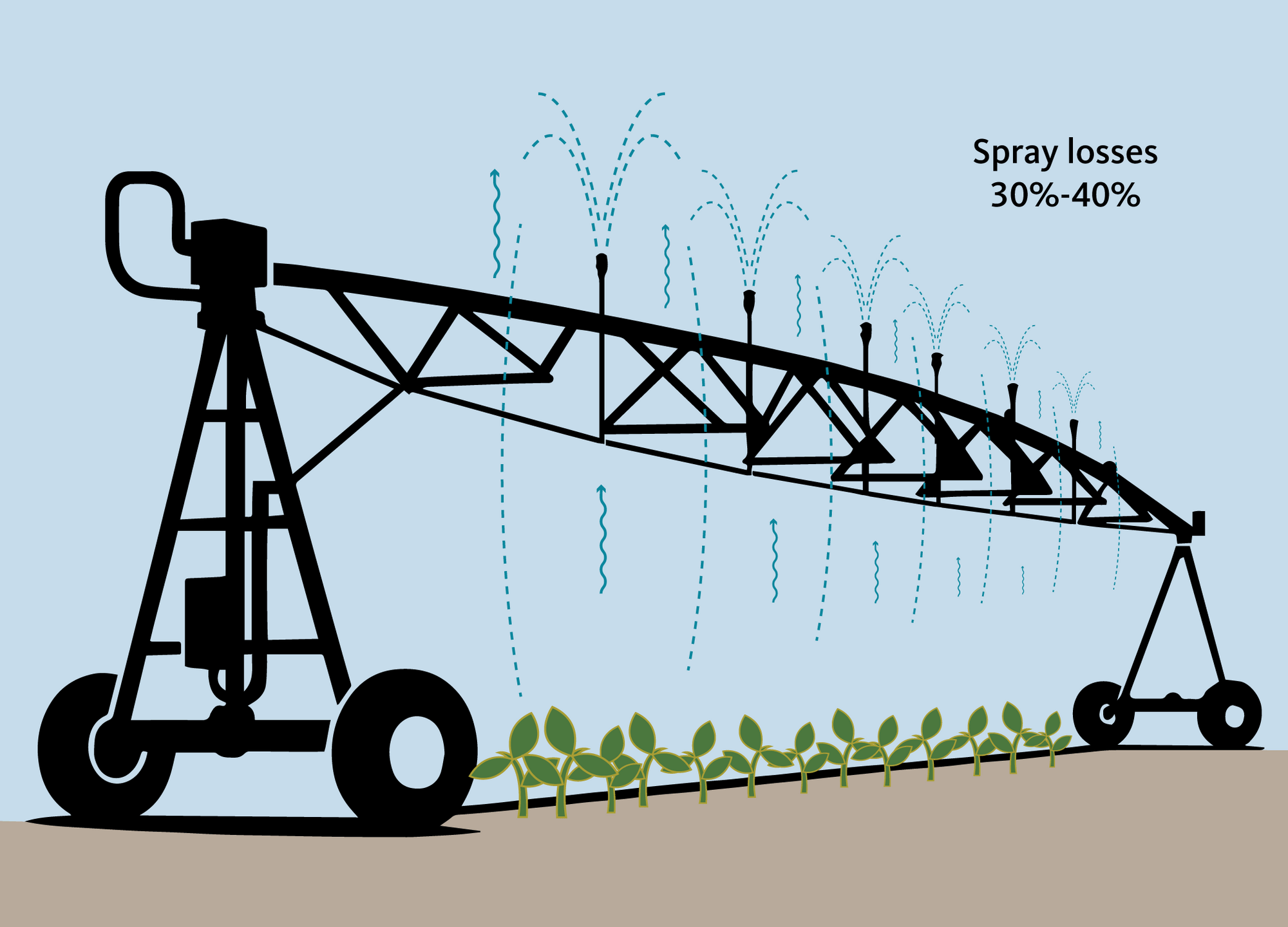
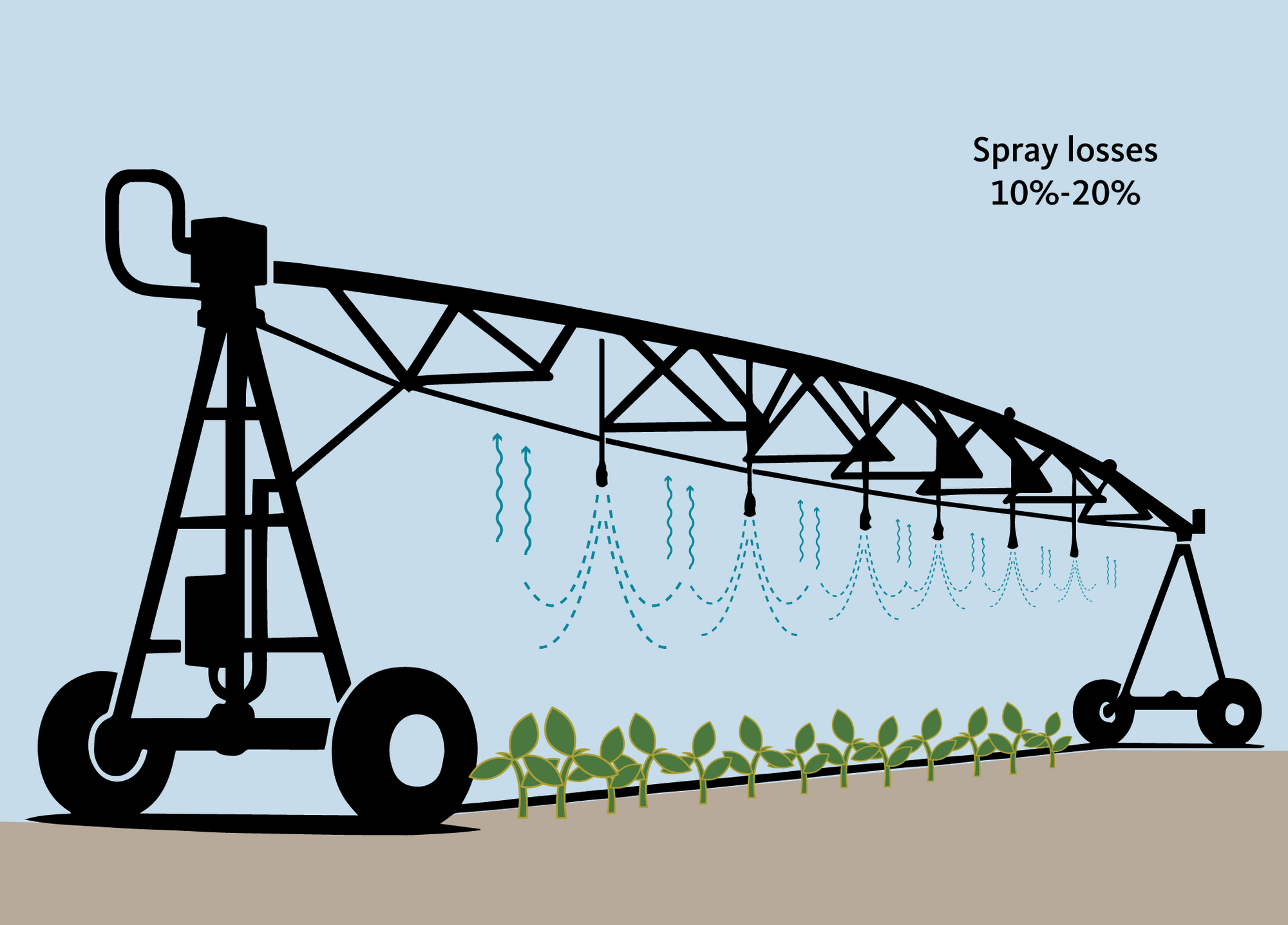
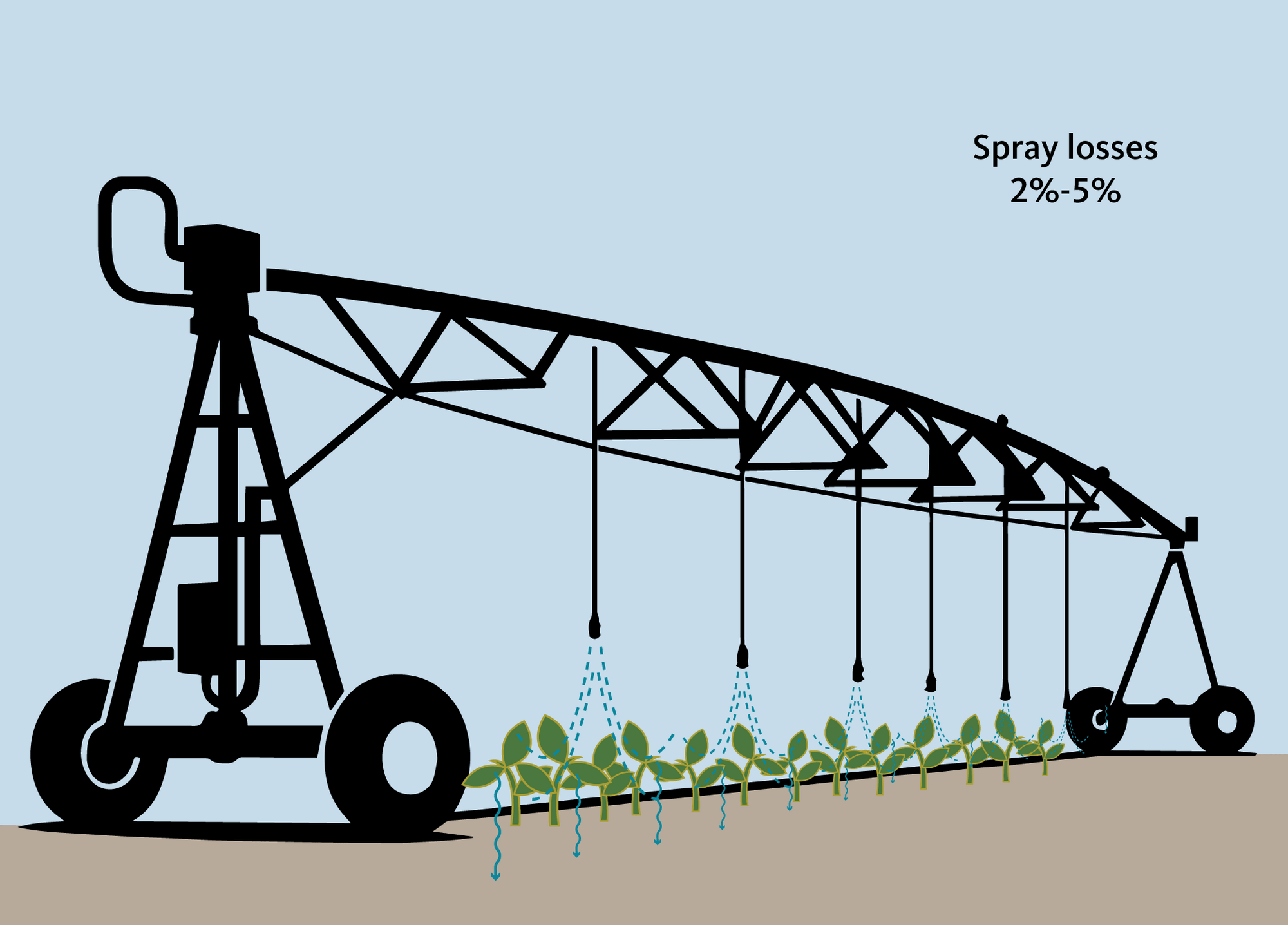
Some people assume that an irrigation system delivers 100% of the applied water directly to the crop. This is rarely the case. A portion of applied water is lost before it can be stored in the root zone due to:
- Deep percolation below the root zone.
- Wind drift and evaporation.
- Surface runoff.
- Canopy interception.
- System leaks and operational losses.
- Poor maintenance or aging equipment.
Irrigation application efficiency is defined as the ratio of the water stored in the crop root zone to the total water applied by the irrigation system.
The sidebar on irrigation systems and their efficiency presents typical application efficiency ranges for common irrigation systems.
In general:
- Newer systems tend to operate at higher efficiency levels.
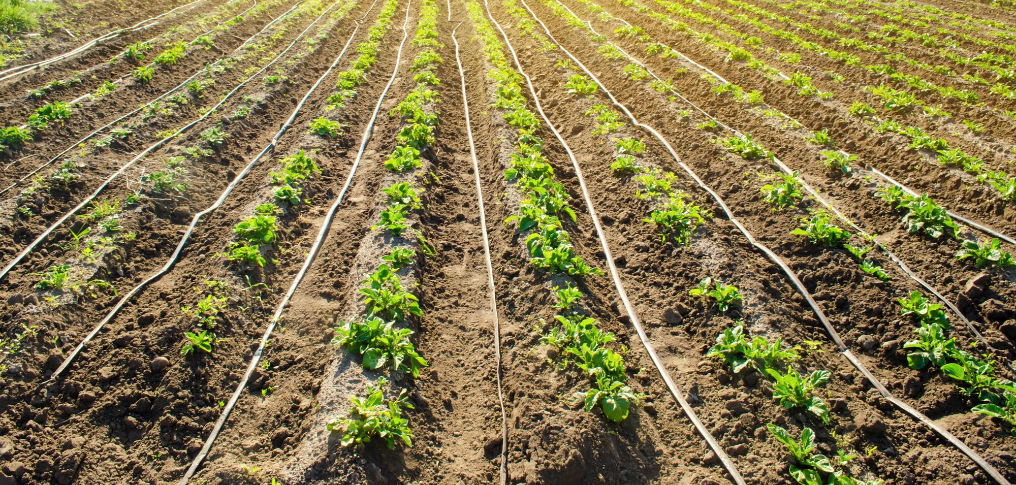
- Microirrigation systems (such as drip) typically achieve the highest efficiencies because water is applied directly to the root zone.
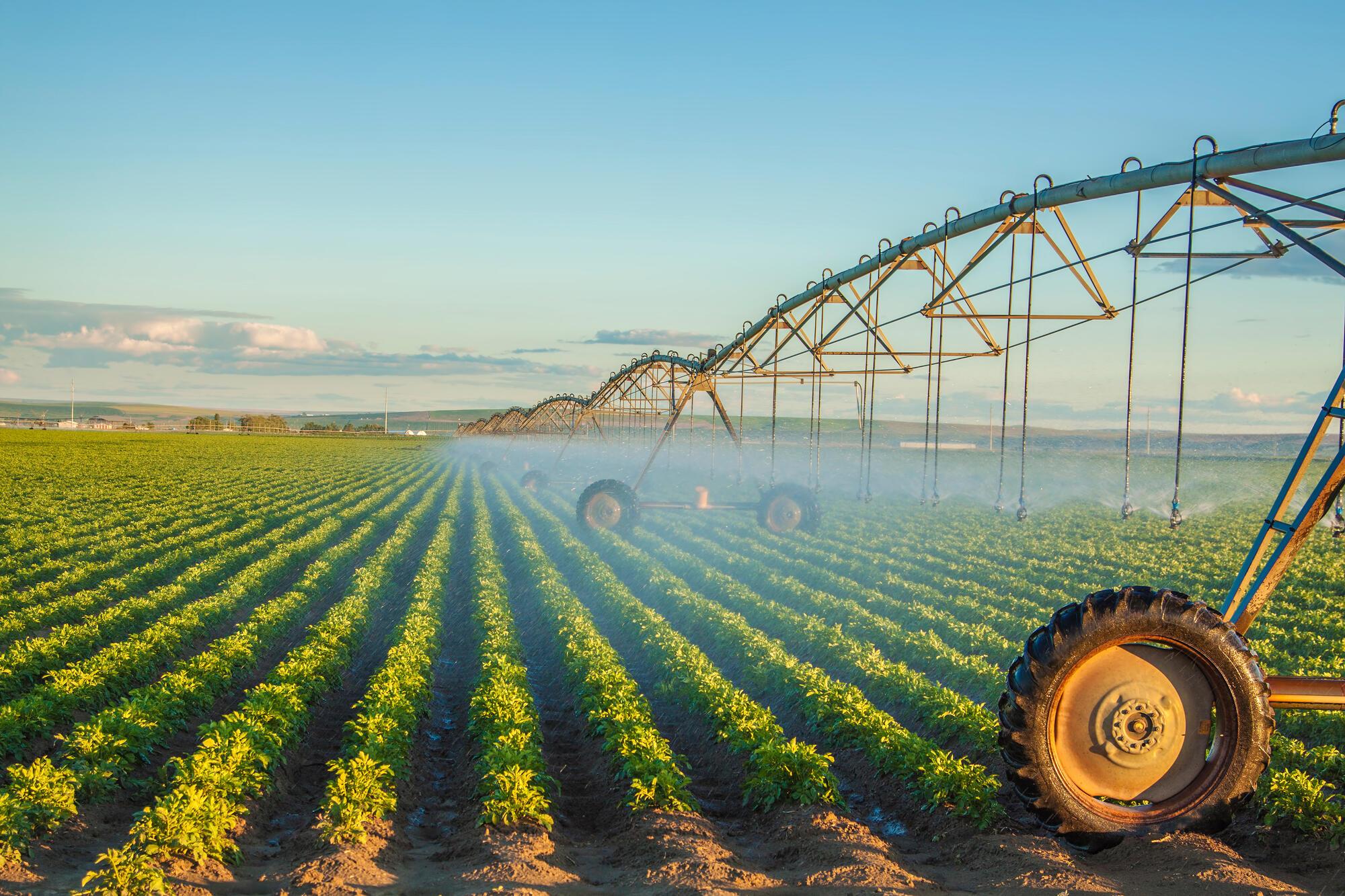
- Sprinkler systems provide moderate efficiency depending on pressure, wind and management.
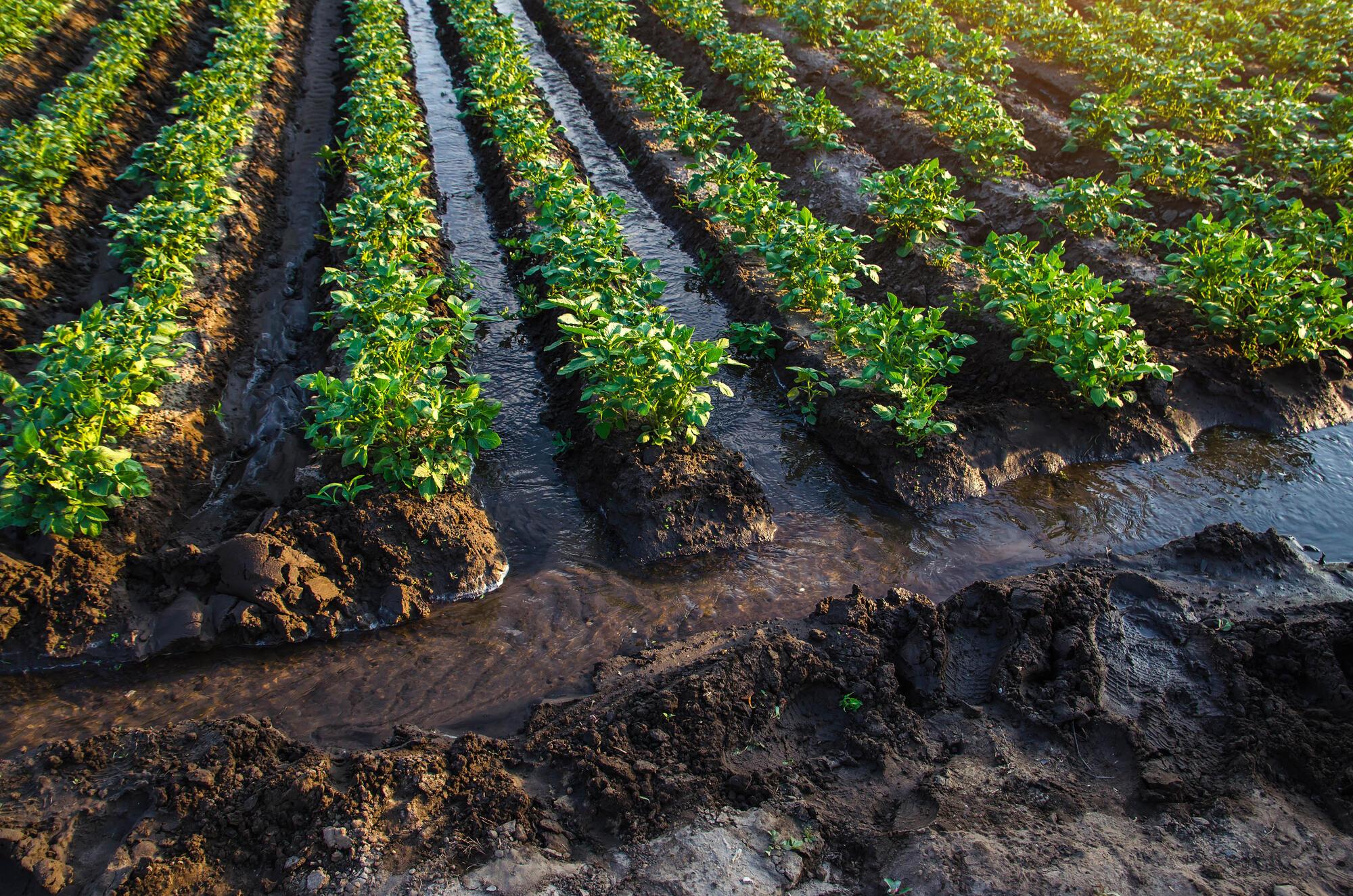
- Surface irrigation systems often have lower efficiency due to runoff and deep percolation losses.
System efficiency is influenced by:
- Design and installation.
- Operating pressure.
- Field slope and soil infiltration characteristics.
- Wind conditions.
- Maintenance and system age.
- Management practices.
Efficiency typically declines over time as systems wear, often by 10%–15% without proper maintenance. Regular inspection, pressure regulation, and timely component replacement help maintain efficiency and reduce both water and energy costs.
Putting it all together!
Now that you have assembled the key pieces of information described above, you can begin improving your irrigation water management. The first step is determining your current net water application depth (inches) — the amount of water stored in the soil after accounting for system efficiency.
This can be calculated using the following formula:
Net water applied (inches) = Net time (hr) × Flow rate (gpm) × 96.3 × System efficiency/Irrigated area (sq ft)
The constant 96.3 converts gallons per minute and hours into inches of water applied over a given area.
Calculating your net water application
Suppose you are operating an older wheel line system that runs for 11.5 hours per set. The riser spacing is 60 feet, sprinkler spacing is 40 feet and the nozzle size is 11/64 inch operating at 60 psi.
From earlier examples, you know:
- Available water in the effective root zone: 2.8 inches (Example 1)
- MAD: 1.7 inches (Example 2)
- Flow rate at 60 psi: 6.6 gpm (Example 3)
- System efficiency: 65% (0.65) (Table 4)
The irrigated area per set is 60 ft × 40 ft = 2,400 sq ft
Applying the formula
11.5 hrs. × 6.6 gpm × 96.3 × 0.65/2,400 sq ft = 1.9 inches
Your system applies 1.9 inches of water per set
What this means
You only need 1.7 inches to refill the soil profile to field capacity, which means the system is applying 0.2 inches too much water.
Over time, this excess irrigation can lead to deep percolation losses, nutrient leaching, increased pumping costs and reduced irrigation efficiency.
In other words, the bucket is overflowing.
To better match crop water needs, you could:
- Reduce set time.
- Install smaller nozzles.
- Adjust operating pressure.
- Improve system efficiency through maintenance.
Calculate net water application on other sprinkler systems
Center pivot and linear move
For pivots and linears, use the total system flow rate (sum of all nozzle flows) and the total irrigated area.
Center pivot and linear system
Unlike the wheel line example above, the pivot formula uses the total system flow (sum of all nozzle discharges) and the entire irrigated area covered during one complete revolution (Note: 1 acre = 43,560 square feet).
Given:
- Pivot rotation time: 24 hours
- Total system flow rate: 247 gpm
- Field area: 33 acres (1,437,480 sq ft)
- Application efficiency: 90% (0.90)
- Conversion factor: 96.3
Net water applied in = 24 hr × 247 gpm × 96.3× 0.90/1,438,480 sq ft
Net water applied (in) = 0.36 inches per revolution
Stationary big gun sprinkler
A stationary big gun applies water to a fixed area for a set time. Net depth applied depends on the sprinkler flow rate, set time, application efficiency and the area covered by the sprinkler spacing.
Given:
- Set time: 12 hours
- Sprinkler flow rate: 80 gpm
- Sprinkler spacing: 120’ x 120’ spacing (14,400 sq ft)
- Application efficiency: 50% (0.50)
- Conversion factor: 96.3
Net water applied in = 12 hr × 80 gpm × 96.3 × 0.50/14,400 sq ft
Net water applied (in) = 3.2 inches per set
Traveling big gun sprinkler
A traveling gun applies water as it moves across the field. Net depth applied depends on the sprinkler flow rate, application efficiency, travel speed and lane spacing.
Given:
- Sprinkler flow rate: 300 gpm
- Application efficiency: 60% (0.60)
- Travel speed (S): 0.4 ft/min
- Lane spacing (W): 250 ft
- Conversion factor: 1.6
Net water applied (in) = 300 gpm × 1.6 × 0.60/0.4ft/min × 250ft
Net water applied (in) = 2.9 inches applied
Micro/drip system
For drip systems, net depth applied is based on emitter discharge, application efficiency and emitter spacing (row spacing × emitter spacing).
Given:
- Emitter flow rate: 1 gal/hr (gph)
- Application efficiency: 95% (0.95)
- Drip row spacing (SR): 24 in
- Emitter spacing (SE): 4 in
- Conversion factor: 231
Net water applied (in) = 231 × (1 gph × 0.95/24 in × 4 in)
Net water applied (in) = 2.28 inches applied
Calculating the correct set time
You can also rearrange the equation to determine how long you should irrigate to replace only the water that has been depleted.
Set time (hr) = Net water needed (in) × Irrigated area (sq ft)/Flow rate (gpm) × 96.3 × System efficiency
Using the same example
1.7 in × 2,400 sqft/6.6 gpm× 96.3 × 0.65 = 9.8 hours
You should irrigate for approximately 10 hours per set to refill the plant-available water without overirrigating.
Important note:
This approach can be used for any sprinkler system once you know the flow rate, irrigated area and efficiency.
This process provides a quantitative foundation for irrigation scheduling and allows producers to adapt irrigation decisions to soil, crop and weather conditions.
Advancing your water-management skills
The amount of water used by a crop depends on the rate of water loss to the atmosphere through evaporation from the soil and transpiration from the plant. Together, these processes are referred to as evapotranspiration. Evapotranspiration represents the consumptive use of water by the crop and varies throughout the growing season in response to crop growth stage, temperature, solar radiation, wind, humidity and soil moisture conditions.
Now that you can determine how much water the soil can hold (the “bucket”) and how much water your irrigation system applies, irrigation scheduling becomes a matter of balancing soil water depletion and refilling the root zone before the crop reaches its maximum allowable depletion.
This can be accomplished using climate data, soil moisture monitoring or a combination.
Climate data
Climate data from AgriMet provide daily estimates of reference evapotranspiration (ETo). Reference evapotranspiration reflects atmospheric water demand for a well-watered reference crop (grass or alfalfa). Crop evapotranspiration (ETc) is calculated by multiplying reference evapotranspiration by a crop coefficient (Kc) that accounts for crop type and growth stage.
ETc = ETo × Kc
AgriMet crop water use charts incorporate these relationships and are updated daily based on weather conditions from the previous day. These data allow irrigators to track how much water has been removed from the soil profile.

To determine soil water depletion using ETc:
Soil water depletion = Previous depletion + ETc - Rain - Net irrigation applied
When cumulative depletion approaches the crop’s maximum allowable depletion, irrigation should be applied to refill the root zone to near field capacity without exceeding soil infiltration capacity.
The goal is to transition from a constant set time to a variable irrigation schedule that responds to crop water use and weather conditions.
See step-by-step guidance for accessing AgriMet data.
Scheduling irrigations
Irrigation scheduling optimizes the timing and amount of irrigation to prevent both overirrigation and crop stress. Methods range from manual recordkeeping to automated smartphone applications.
|
Field |
Withdrawals |
Deposits |
Balance |
Notes |
|
|---|---|---|---|---|---|
|
A |
B |
C |
D |
E |
F |
|
Date(month/day) |
Crop water use (ET) (inches) |
Net irrigation (inches) |
Effective rainfall in inches (subtract 0.15 inches from measured rainfall) |
Available soil water (previous E – B + C + D) (inches) |
Minimum balance 4.3 in. Observed/measured soil moisture level or depletion. Data and amount of next irrigation. |
|
Example entries for daily values |
|||||
|
7/1 |
- | - | - | 5.42 | Measured soil water |
|
7/2 |
0.18 | 0 | 0 | 5.24 | |
|
7/3 |
0.20 | 0 | 0.45 | 5.34 | |
|
7/4 |
0.17 | 0 | 0 | 5.17 | |
|
7/5 |
0.22 | 0 | 0 | 4.95 | |
|
7/6 |
0.24 | 0 | 0 | 4.71 | |
|
7/7 |
0.26 | 0 | 0 | 4.45 | Irrigate 1.2 in. (net) on 7/8 |
|
7/8 |
0.22 | 1.2 | 0 | 5.32 | |
|
7/9 |
0.17 | 0 | 0 | 5.36 | |
1. Checkbook method
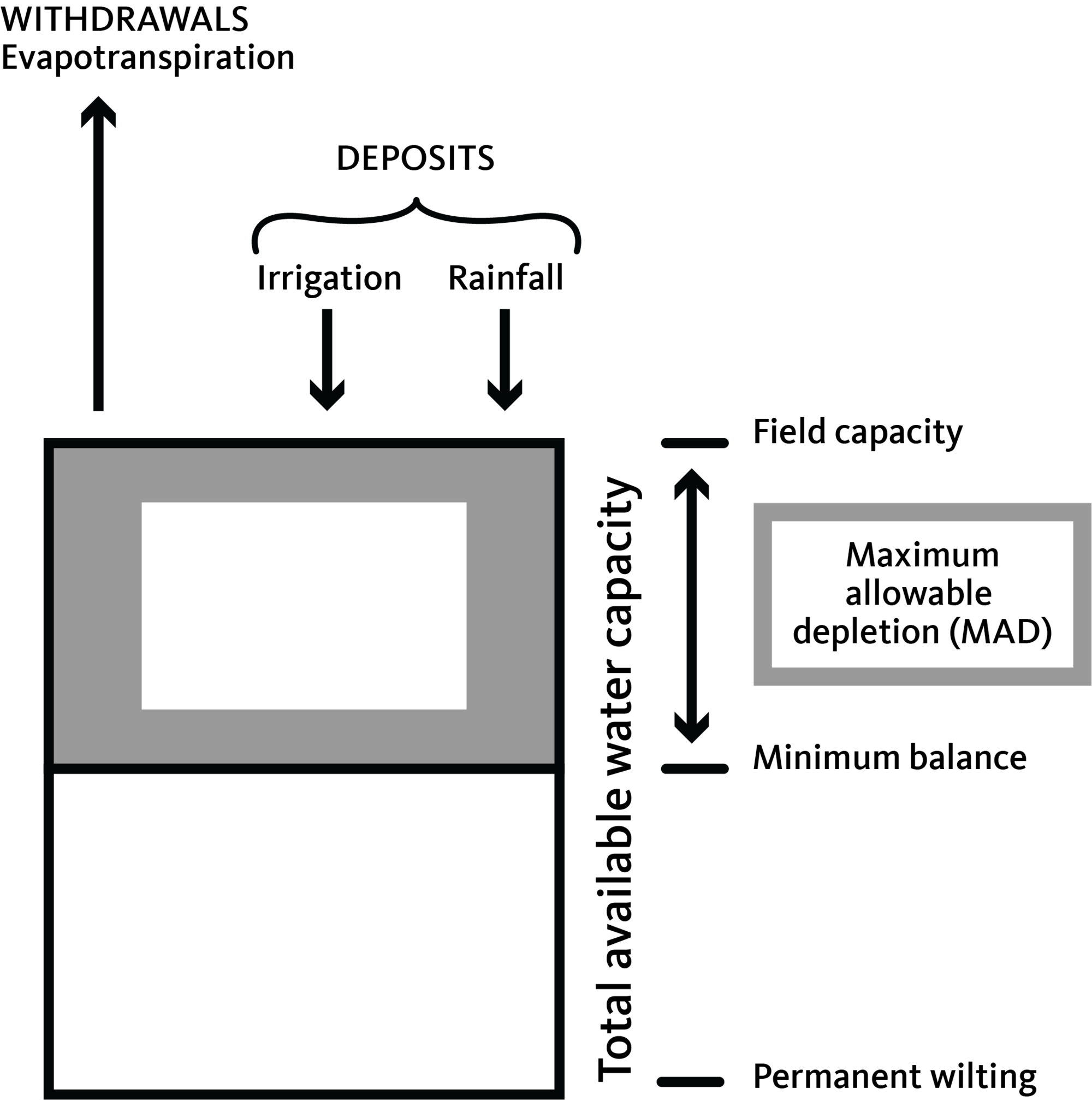
The checkbook method (Figure 8) tracks soil water content much like a financial account:
- Available soil water represents the account balance.
- Evapotranspiration, the water that evaporates from the soil surfaces and transpires from the plants, represents withdrawals.
- Irrigation and rainfall represent deposits.
- Maximum allowable depletion represents the minimum balance.
Therefore, as water is removed from the soil (withdrawals) and soil water depletion reaches the maximum allowable depletion limit (minimum balance), irrigation is required to restore soil moisture toward field capacity (deposit). When irrigation doesn’t occur, the crop might begin to experience water stress that could lead to yield losses. (This would be considered an overdraft on your account.)
This method requires knowledge of:
- Soil available water capacity
- Effective rooting depth
- Maximum allowable depletion
- Irrigation system efficiency
- Daily evapotranspiration, or ETc
- Precipitation
Note: Weather and ETc data can be obtained through AgriMet.
Irrigation scheduling record books are available through local Natural Resources Conservation Service offices.
2. Smartphone-based irrigation scheduling tools
With technological advancements, tracking evapotranspiration and determining when to irrigate has become easier.
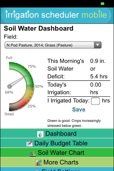
The Irrigation Scheduler Mobile application is one of several automated tools available (Figure 9). It integrates crop information, soil characteristics and AgriMet climate data to track depletion and recommend when and how much to irrigate.
Smart irrigation tools allow irrigators to:
- Automate ETc tracking
- Forecast irrigation timing
- Display seasonal water use
- Improve labor efficiency and recordkeeping
To know more about the Irrigation Scheduler Mobile application and how to use it, see the training video.
A user’s guide is also available.
Monitoring
Tracking the consumptive use of the crop is only one part of the equation for irrigation scheduling. Always pair climate-based scheduling with field verification.
Soil moisture monitoring provides direct measurement of root zone water status and validates scheduling assumptions.
Monitoring methods
Look-and-feel method (qualitative field assessment)
This is a simple method that can allow you to physically examine soil moisture in the field and correlate field observations with the available soil water value in your checkbook or irrigation scheduling tool.
Estimating Soil Moisture by Feel and Appearance is an excellent resource to determine soil moisture for various soil textures in the field.
In-field sensors
Portable or stationary sensors are available to determine, in near real time, the soil moisture or soil matric potential within the effective root depth of your crop.
- Tensiometers
- Capacitance or TDR soil moisture sensors
- Portable or permanently installed probes
Monitoring soil and crop conditions allows growers to:
- Confirm irrigation depth is reaching intended root depth
- Detect over- or underirrigation
- Adjust for soil variability within fields
Combining climate data with soil moisture monitoring provides the most robust irrigation management approach. To know more about these devices, consult your local irrigation supply dealer.
Satellite data
Satellite-based evapotranspiration tools combine satellite imagery and weather data to estimate crop water use at the field scale. These tools estimate actual evapotranspiration (ETa), which represents modeled crop water use under existing field conditions.
One widely used platform is OpenET. OpenET provides satellite-based evapotranspiration estimates at approximately 30-meter resolution and can be used to:
- Track seasonal crop water use
- Compare water use among fields
- Evaluate irrigation performance
- Support water management reporting and conservation planning
Satellite-based evapotranspiration data are particularly useful for assessing cumulative water use and irrigation performance over time. However, satellite-based estimates should complement in-field monitoring. Satellite data represent spatial estimates and may not capture small-scale soil variability, irrigation non-uniformity or short-term moisture stress. For best results, satellite evapotranspiration data should be used in combination with local weather data, soil moisture or any other in situ measurements.
Effective irrigation scheduling combines an understanding of soil water storage, crop water use, irrigation system performance and irrigation efficiency with climate data, satellite-based evapotranspiration estimates and in-field monitoring. By integrating these tools, growers can apply the right amount of water at the right time — improving crop yield and quality, conserving water resources and reducing pumping energy and input costs.
References and resources
Broner, I. February 2005. Irrigation Scheduling 4.708, Colorado State University Extension.
Melvin, Steven R., and C. Dean Yonts. 2009. Irrigation Scheduling Checkbook Method, EC709. University of Nebraska Extension.
Montana State University Extension. September 1990. Irrigation Water Management: When and How Much to Irrigate, MT 8901.
Morris, Mike, and Vicki Lynne. 2006. Measuring and Conserving Irrigation Water, ATTRA-National Sustainable Agriculture Information Service.
Morris, Mike. 2023. The Irrigator’s Pocket Guide, National Center for Appropriate Technology.
Natural Resources Conservation Service. September 1997. National Engineering Handbook, part 652 Irrigation Guide, chapter 9 Irrigation Water Management.
Natural Resources Conservation Service. September 1997. National Engineering Handbook, part 623 Irrigation Guide, chapter 2 Soil Plant Water Relationship.
North Dakota State University, Irrigation Scheduling..
Peters, R. Troy, Gerrit Hoogenboom and Sean Hill. Simplified Irrigation Scheduling on a Smartphone or Web Browser.
U.S. Department of Agriculture, Montana Natural Resources Conservation Service. 2023. Irrigation Scheduling Recordbook.
Washington State University Extension. Scientific Irrigation Scheduling, EM4825.
About the authors


